arviz_plots.plot_ppc_interval#
- arviz_plots.plot_ppc_interval(dt, var_names=None, filter_vars=None, group='posterior_predictive', coords=None, sample_dims=None, point_estimate=None, ci_kind=None, ci_probs=None, plot_collection=None, backend=None, labeller=None, aes_by_visuals=None, visuals=None, stats=None, **pc_kwargs)[source]#
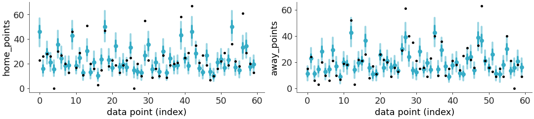
Plot posterior predictive intervals with observed data overlaid.
Displays observed data as a point and predicted data as a point estimate plus two credible intervals.
- Parameters:
- dt
xarray.DataTree Input data. It should contain the
posterior_predictiveandobserved_datagroups.- var_names
strorlistofstr, optional One or more variables to be plotted. Prefix the variables by ~ when you want to exclude them from the plot.
- filter_vars{
None, “like”, “regex”}, default=None If None, interpret var_names as the real variables names. If “like”, interpret var_names as substrings of the real variables names. If “regex”, interpret var_names as regular expressions on the real variables names.
- group
str Group to be plotted. Defaults to “posterior_predictive”. It could also be “prior_predictive”.
- coords
dict, optional Coordinates of var_names to be plotted.
- sample_dims
stror sequence of hashable, optional Dimensions to reduce unless mapped to an aesthetic. Defaults to
rcParams["data.sample_dims"]- point_estimate{“mean”, “median”, “mode”}, optional
Which point estimate to plot for the predictive distribution. Defaults to rcParam
stats.point_estimate.- ci_kind{“hdi”, “eti”}, optional
Which credible interval to use. Defaults to
rcParams["stats.ci_kind"].- ci_probs(
float,float), optional Indicates the probabilities for the inner (twig) and outer (trunk) credible intervals. Defaults to
(0.5, rcParams["stats.ci_prob"]). It’s assumed thatci_probs[0] < ci_probs[1], otherwise they are sorted.- plot_collection
PlotCollection, optional - backend{“matplotlib”, “bokeh”, “plotly”, “none”}, optional
- labeller
labeller, optional - aes_by_visualsmapping of {
strsequence ofstrorFalse}, optional Mapping of visuals to aesthetics that should use their mapping in
plot_collectionwhen plotted.- visualsmapping of {
strmapping or bool}, optional Valid keys are:
trunk, twig -> passed to
ci_bound_yobserved_markers -> passed to
point_yprediction_markers -> passed to
point_yxlabel -> passed to
labelled_xylabel -> passed to
labelled_ytitle -> passed to
labelled_titledefaults to False
- statsmapping, optional
Valid keys are:
trunk, twig -> passed to eti or hdi
point_estimate -> passed to mean, median or mode
- **pc_kwargs
Passed to
arviz_plots.PlotCollection.grid
- dt
- Returns:
See also
plot_ppc_distPlot 1D marginals for the posterior/prior predictive and observed data.
plot_ppc_rootogramPlot ppc rootogram for discrete (count) data
plot_forestPlot forest plot for posterior/prior groups.
Examples
Plot posterior predictive intervals for the radon dataset, with custom styling.
>>> from arviz_base import load_arviz_data
>>> import arviz_plots as azp
>>> azp.style.use("arviz-variat")
>>> data = load_arviz_data("rugby")
>>> pc = azp.plot_ppc_interval(data)